Doppler Echocardiography
Check out this great resource A Practical Approach to Transesophageal Echocardiography
Why Doppler Why Now?
Christian Doppler in 1842 presented findings in astronomy that would go on to be dubbed the Doppler effect or Doppler shift. The original paper was titled: “Uber das farbige Licht der Doppelsterne und einiger anderer Gestirne des Himmels” or “ On the colored light of the binary stars and some otehr stars of the heavens.” His observations focused on the change in the frequency of light relative to an observer who is moving relative to the source of the wave. This is commonly seen in astronomy and called the red shift as objects move farther away from earth, their colors move to the red end of the visual spectrum. A more approachable example on earth is a siren on an emergency vehicle as it moves toward you and then away from you as it passes by. The pitch gets higher as the siren gets closer and lower as it moves away.
The equation for the Doppler effect when the observer is stationary and the source is moving:
\[{f} = {c \pm v_r \over c \pm v_s}{f_0}\]f is the observed frequency and $f_0$ is the original frequency, c is the propagation speed of the waves in the medium, $v_r$ is speed of the receiver or observer while $v_s$ is the speed of the source.
Doppler in Medicine
It took more than 100 years for the Doppler effect to be applied to medicine. 1954 saw the use of Doppler to measure flow velocity in the brain, followed by movements of cardiac structures, and later ultrasound was used to see the heart. By the 1960s ultrasound was being introduced in clinical practice in cardiology. Doppler echocardiography was not used until the 1970s. Now we use color, pulse, tissue, and continuous wave Doppler routinely in the assessment of cardiac function.
When Doppler is applied to medicine applications specifically echocardiography sonographers are able to ascertain many properties using this minimally invasive technique. It is important to remember to ensure that the beam of the Doppler is as parallel as possible to the measured item. The most common items analyzed with Doppler are flow direction, velocity, cardiac output, with some additional applications in obstetrics, and neurology.
In many instances the medical use of Doppler is not synonomous with velocity because the frequency shift is not measured, but in fact the phase shift is measured.
The equation for the Doppler effect in echocardiography:
\[{f} = {2vf_0cos\theta\over c}\]f is the observed frequency and $f_0$ is the original frequency from the ultrasound probe, c is the propagation speed of the ultrasound in the blood, v is the velocity of the red cell target, and $\theta$ is the angle of the ultrasound beam to the vector of blood flow. See the effect of different angles:
$cos90 = 0$ $cos0 = 1$ $cos30 = 0.87$
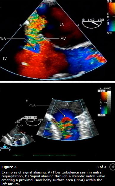
Nyquist Limit
Harry Nyquist was the founder. The principle is $1\over2$ the sampling rate of a signal that is discreetly sampled. If this limit is exceeded red and blue appear side by side due to signal aliasing. This means that turbulance is missed and one will underestimate the lesion. If the limit is set too low false turbulence will be noted and over estimation of the lesion can happen.
Valves and Arterial Flow: 50-70cm/sec
Venous and Intra-atrial Septum: 30-50cm/sec
Color Doppler
Crystals both recieve and transmit signals but rather than focusing on a single point, multiple sample volumes are evaluated along each individual sampling line. Velocities are detected and depicted with blue signals moving away from the probe and red moving toward.
Continuous Wave (CW) Doppler
Two crystals used one for emission and one for receiving. Every velocity along the line of interrogation is recorded. This is useful for very high velocities but is unable to pinpoint from where on the scan line they originate.
Pulse Wave (PW) Doppler
A single crystal is used for both emission and receiving. By knowing the velocity of body tissue the crystal waits for the reflected signal to return thus interrogating a specific area. Distance can make this measurement faulty and directionality of flow will be unknown. This is called aliasing which can also happen when the Nyquist limit is exceeded.
Tissue Doppler
Myocardial wall motion velocities can be interrogated when aimed at a wall rather than blood flow. This can provide diastolic measurements. Assumptions that must be taken into consideration include laminar flow, simultaneous variable measurement, cross sectional areas are perfect circles, areas are fixed and never change. While none of these are true in humans we use these assumptions in order to make meaningful analysis or diagnosis from the echo.
Measurment Techniques
Valve Area
Valve opening areas are important measures for both native valves and determining their degree of stenosis and the same measurement on their artificial counterparts.
Continuity Equation
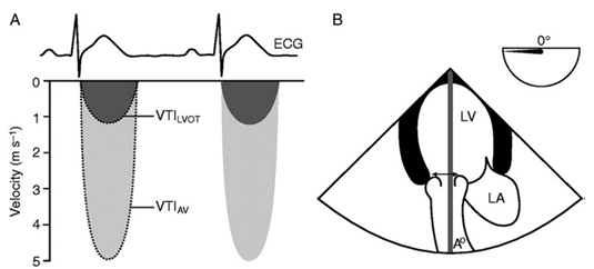
SD = stroke distance SV = stroke volume v = velocity t = time AV = aortic valve CSA = cross sectional area r = radius VTI = volume time integral
In order to find the area of the LVOT the diameter must be measured.
To find the VTI of the aortic valve you need to use CW doppler in the TG LAX view. To find the LVOT VTI you need to use PW Doppler in the TG LAX view. It is possible to find both of the velocities using CW Doppler if the LVOT and AV are lined up. This is called the double envelope technique. The drawback of this technique is that it may overestimate the AV area.
\[SD = v*t = \int_{AV open}^{AV close}vdt\] \[CSA = \pi(r_{LVOT})^2\] \[SV = SD * CSA\]Finally to find the area of the aortic valve you need to substitute VTI for V since volume is travelling through the structures over time:
\[A_1 * V_1 = A_2 * V_2\] \[CSA_{AV} * VTI_{AV} = CSA_{LVOT} * VTI_{LVOT}\] \[{CSA_{AV}} = {CSA_{LVOT} * VTI_{LVOT} \over VTI_{AV}}\]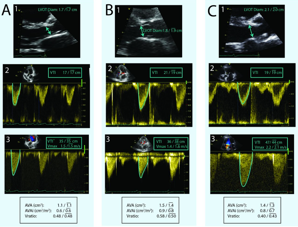 1. is LVOT diameter measurement for CSA, 2. is PW in the LVOT for the VTI, and 3. is CW through the AV for VTI
 Double envelope technique
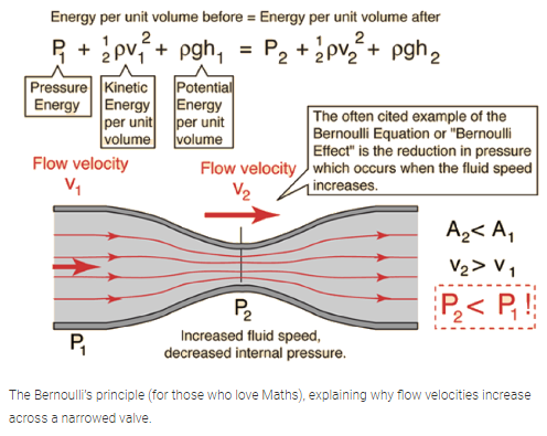
Why the continuity equation and Bernoulli’s equation work:
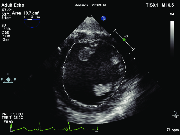
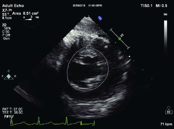
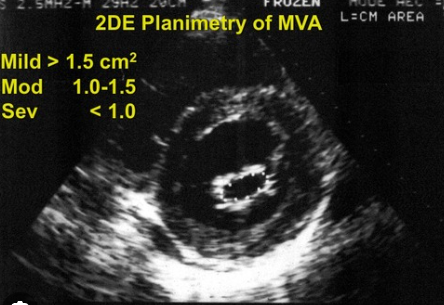
Planimetery
With a good enough view the valve opening can be traced and calculated using the echo software. This is frequently done for the mitral valve using the TG view.
Pressure Gradient
This is measured using the modified or simplified Bernoulli Equation.
Full equation:
The first term deals with convective acceleration, the second term deals with flow acceleration and the final term deals with viscous friction.
\[\Delta P = 0.5 * p(V_2^2 - V_1^2) + \int_1^2 (dv/dt) x ds + R(v)\]Modified equation:
In many cases the volume through the $V_1$ structure is negligable so the simplified version is used. If $V_1$ is > 1.4m/s the modified euqation should be used.
\[\Delta P = 4 (v_2^2 - v_1^2)\]Simplified equation:
\[\Delta P = 4v^2\]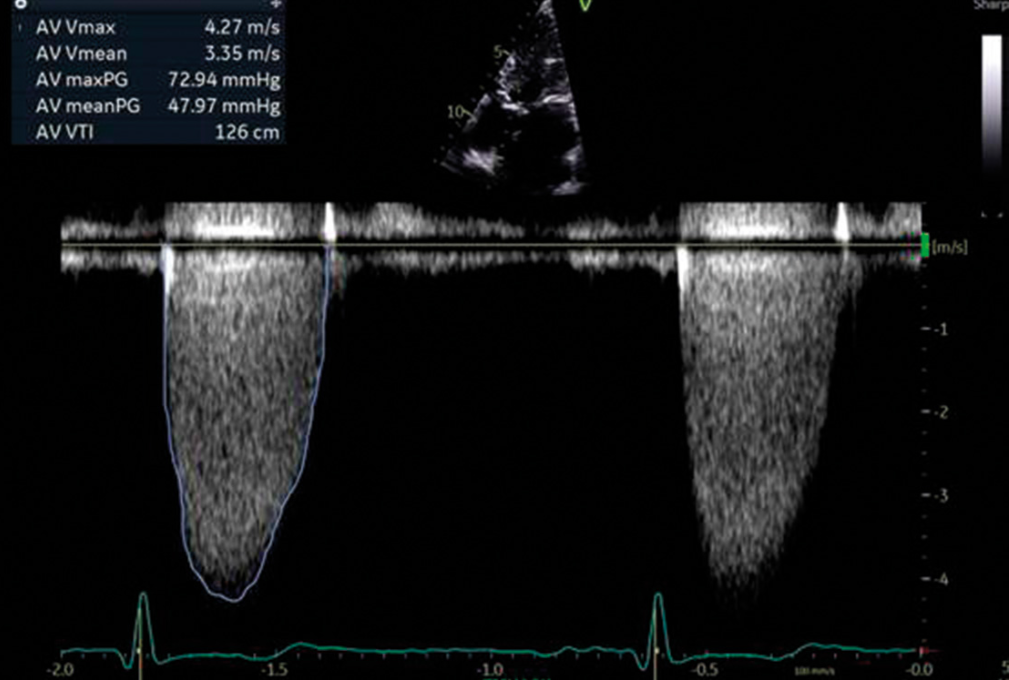
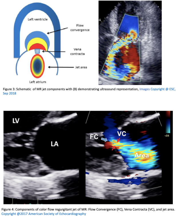
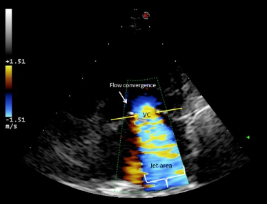
Vena Contracta
This is a measurement of the narrowest portion of a regurgitant jet or where there is flow convergence.
Pressure Half Time
Pressure half time or PHT is the measurement used for mitral valve area or aortic regurgitation. The concept is based on pressure deceleration. PHT is independent of both CO and MR. However it can be underestimated in low flow states. To get a measurement use CW doppler at the mitral opening in early diastole. This will give a velocity tracing. PHT is the measure of the rate of decrease in pressure and the time to decrease to 50% of the peak velocity. As stenosis worsens the PHT increases. Experimental models show a PHT of 220ms eqates to a MVA of 1cm.
Equation to link area and PHT:
\[A = {220 \over PHT}\]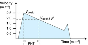
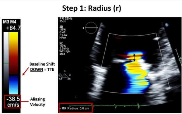
Proximal isovelocity surface area (PISA)
This term describes an idea in physics where, when fluid flows through an orifice all equidistant points towards the orifice exhibit the smae velocities.The velocity increases near the orifice giving the appearance of multiple concentric hemispheres of flow convergence with equal velocity. PISA is commonly used in MV analysis.
PISA flow rate = Regurgitant flow rate
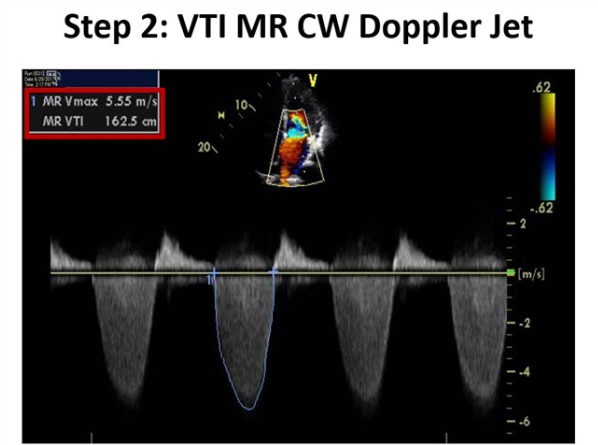
Where $velocity_{PISA}$ is the Nyquist limit, EROA is the effectvie regurgitant orifice area and the MR is mitral regurgitant VTI.
\[CSA_{PISA} * velocity_{PISA} = EROA_{MV} * VTI_{MR}\]You solve for the EROA which is a marker of MR severity and then use it to find the MR volume.
\[Regurgitant volume(MR) = EROA_{MV} * VTI_{MR}\]The above can be time consuming in the OR so a simplified method is below where r is the PISA radius:
\[{EROA_{MR}} = {r^2\over 2}\]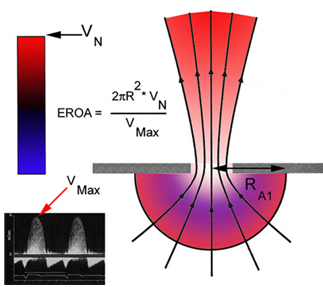
Mitral Regurgitation
- Vena contracta
- Jet area
- PISA
- PW Doppler in the pulmonary veins to assess for flow reversal
| Measurement | Mild | Moderate | Severe |
|---|---|---|---|
| Vena Contracta (mm) | < 3 | 3-6.9 | > 7 |
| Jet area / LA area | < 20 | 20-40 | > 40 |
| PISA radius (mm) | < 4 | 4-10 | > 10 |
| Regugitant volume (ml) | < 30 | 30-59 | > 60 |
| Regurgitant fraction % | < 30 | 30-49 | > 50 |
| EROA (cm^2) | < 0.2 | 0.2-0.4 | > 0.4 |
Mitral Stenosis
- Planimetry (Deep TG) valve area
- Pressure gradient
- PHT
- PISA
| Measurement | Normal | Mild | Moderate | Severe |
|---|---|---|---|---|
| Valve Area ($cm^2$) | > 2 | 1.5-2 | 1-135 | < 1 |
| Mean Pressure Gradient | < 5 | 5-10 | > 10 | |
| Pressure Half Time (ms) | < 71-139 | 140-219 | > 219 | |
| Indexed Valve Area $cm^2 / m^2$ | 2 | > 0.85 | 0.6-0.85 | < 0.6 |
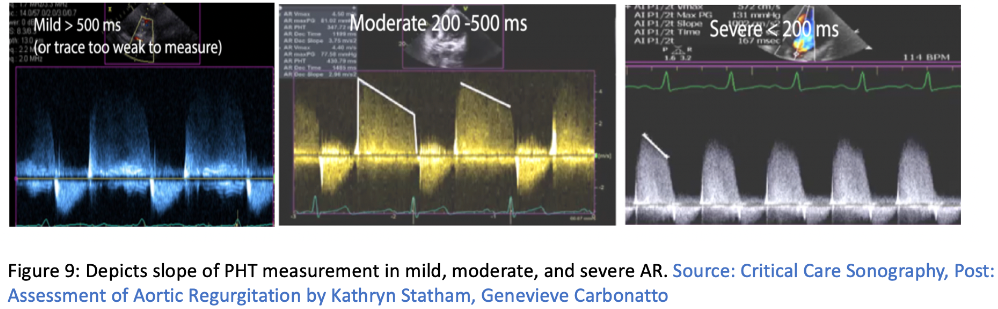
Aortic Regurgitation
- Vena contracta
- Jet/ LVOT ratio
- PHT
- PISA
| Measurement | Mild | Moderate | Severe |
|---|---|---|---|
| Vena Contracta (mm) | < 3 | 3-6 | > 6 |
| Jet area / LVOT area | < 4 | 4-6 | > 60 |
| PHT (ms) | > 500 | 500-200 | <200 |
| Regugitant volume (ml) | < 30 | 30-59 | > 60 |
| Regurgitant fraction % | < 30 | 30-49 | > 50 |
| EROA (cm^2) | < 0.1 | 0.1-0.29 | > 0.3 |
Aortic Stenosis
- Peak velocity (CW)
- Mean gradient
- Valve area
- Dimensionless index (attempts to compensate for CO and other variables)
| Measurement | Aortic Sclerosis | Mild | Moderate | Severe |
|---|---|---|---|---|
| Valve Area ($cm^2$) | 2.6-3.5 | > 1.5 | 1-1.5 | < 1 |
| Mean Gradient (mmHg) | < 10 | < 20 | 20-40 | > 40 |
| Indexed Valve Area $cm^2 / m^2$ | 2 | > 0.85 | 0.6-0.85 | < 0.6 |
| Peak velocity of flow (m/sec) | 2.6 | < 2.6-3 | 3-4 | > 4 |
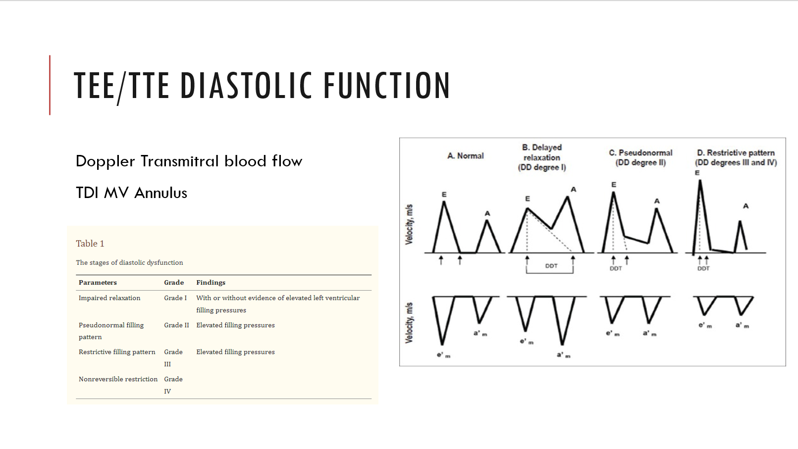
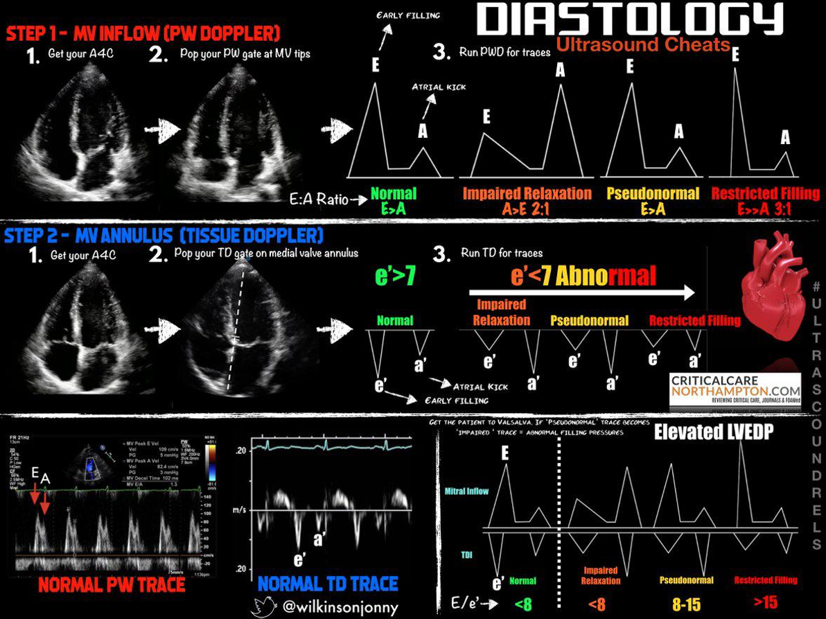
LV Diastolic Function Assessment
Using Doppler to diagnosis heart failure with preserved ejection fraction requires PW Doppler at the mitral annulus and/or tissue Doppler at the medial mitral annulus. The ratios and velocities are then used to extrapolate diastolic dysfunction.
Grade 1 through 4. Grade 1 is associated with 8x increase in all cause mortality within 5 years!
If e’ is < 7 (MV tissue doppler), or the E/e’ is more than 8, or if the E:A ratio is more than 2:1 there is diastolic dysfunction
Examples of diastology with traditional methods:
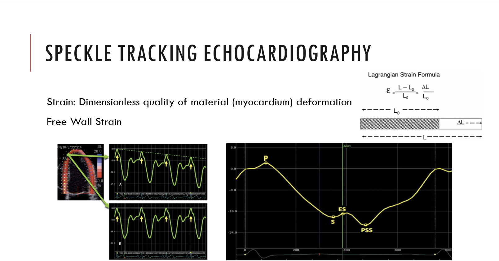
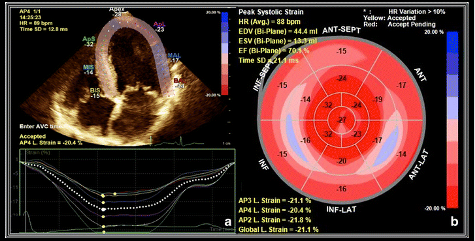
Examples of speckle tracking:
Hypertrophy
Remember LV thickness corresponds to LV mass and a 1mm error can through off the LV mass by 15g or more!
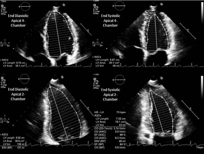
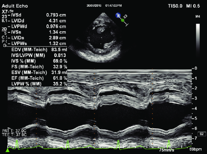
LV Systolic Function
In normal hearts the Teicholz equation is accurate, but for hearts suffering from infaractions past or present the disc method using Simpson’s Rule is preferred.
V = LV Volume D = LV diameter
\[V = {7D^3 \over 2.4 + D}\]Simpson’s Method
Discs are used to determine the ejection fraction.
Fractional Shortening in M-Mode
The software will calculate the fractional shortening and ejection fraction.
Fractional Area Change
The software will calculate the area change and ejection fraction.